How To Sum Negative Numbers In Google Sheets
SumDD If you just want to sum a few numbers you can use the SUM function as below. To sum the total number of units sold enter the following functions into cells E2 and F2 respectively.
Replace Negative Values With Zero In Excel Google Sheets Automate Excel
You can format a number to a fraction in two ways.

How to sum negative numbers in google sheets. In the pop-up window 1 select Format only cells that contain in Rule type options 2 choose less than 3 enter 0 in the Value box and 4 click Format. If the latter is negative this returns a 0. This will open the Conditional formatting rules pane on the right Click on the.
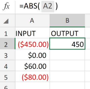
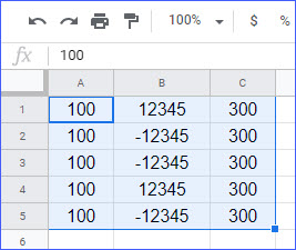
Luckily Google Sheets includes an ABS function so that you can quickly get absolute values for negative numbers without editing their cells. Select the range of cells where you want to make negative numbers red and in the Ribbon go to Home Conditional Formatting New Rule. It seems when entering a hyphens - followed by a number Sheets automatically converts the content of the Cell to a number type.
Using the custom number formatting menu option. Some text The second rule which comes between the first and second semi-colons tells Google Sheets how to display negative numbers. Select the cell or the data range with the numbers that you want to format.
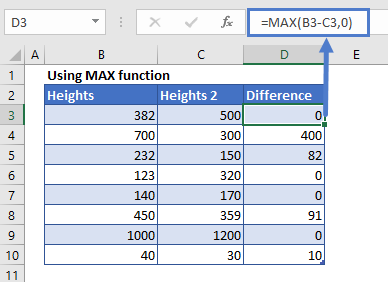
MAX0SUMA1A7-70 It returns the highest value in a range of numbers. In this case 0 or whatever the value of SUBA1A7 - 70 is. Using the Text function.
Its a basic function that you can enter with this. While the former retains the number format the latter converts the number to a text string. 14 Metrics That Every CEO Needs to Knowhttpswwwfinancialgpscocopy-of-free-exclusive-e.
Click on the link below to get our free exclusive eBook today. This would return 250000. SUMIF ARRAYFORMULA FIND text range 1 sum_range Supposing you have a list of order numbers in A5A13 and corresponding amounts in C5C13 where the same order number appears in several rows.
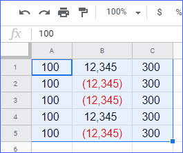
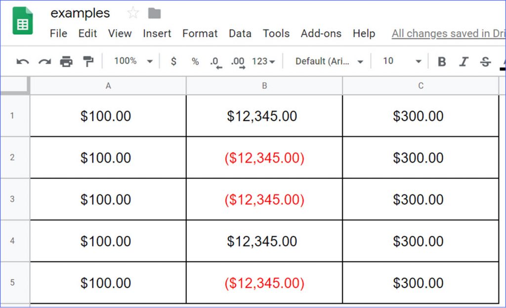
Sum2502502000 Type this formula in any cell. You can format them either in red or in parentheses so you can easily find them after. C16 is the category name lets call it Transfers.
Select the cells in which you want to highlight the negative numbers Click the Format option in the menu Click on Conditional Formatting. The first rule which comes before the first semi-colon tells Google Sheets how to display positive numbers. Opening Sheets in browser on Windows10 Laptop.
The teal is the column holding different values some positive some negative. Two Methods to Format Numbers as Fractions in Google Sheets. To do this we will use another column to write a formula for adding the negativ.
By default the negative numbers are in black with the negative sign. The purple is the column holding different categories one of them being Transfers. To Sum column D use this formula in any other column.
Format for negative numbers 000. As part of this conversion the hyphens - is converted to a different type of Dash resemblling an en dash. You enter the target order id in some cell say B1 and use the following formula to return the order total.
Below are the steps to show negative numbers in red in Google Sheets. This way it takes all the values that match up with the category C16 and sums it up. How to Sum an Entire Column in Google Sheets.
If you get a file with positive number performing calculations is not hard but if the values are mixed with positive and negative numbers it might be a pro. Click the Format tab from the ribbon and click the Number command from the drop-down list. In this video we will add negative values to non-adjacent cells in a column.

Replace Negative Values With Zero In Excel Google Sheets Automate Excel
Excel Formula Change Negative Numbers To Positive Excelchat

Excel Formula Count Cells That Contain Negative Numbers Exceljet
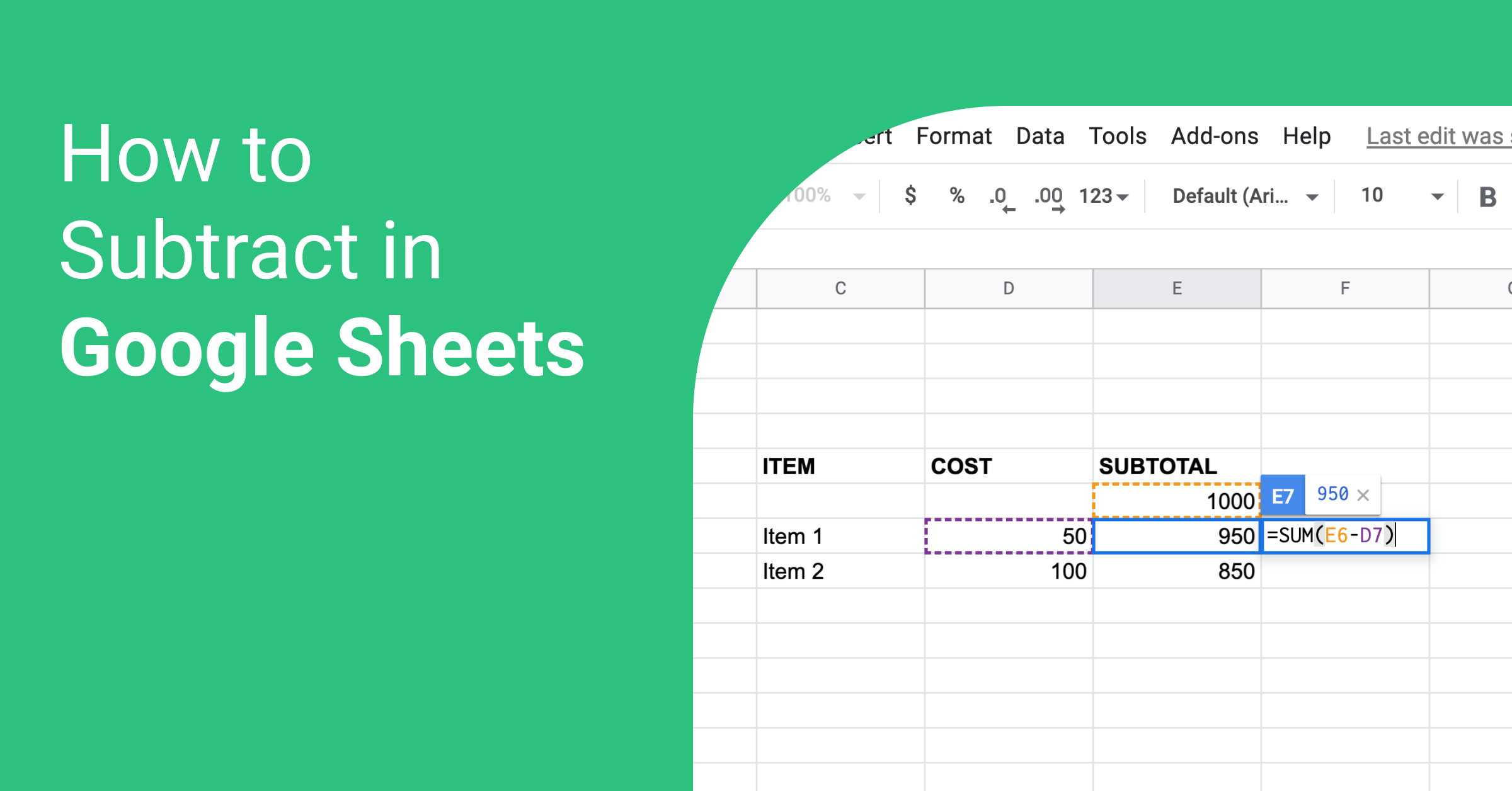
How To Subtract In Google Sheet Visual Tutorial Blog Whatagraph

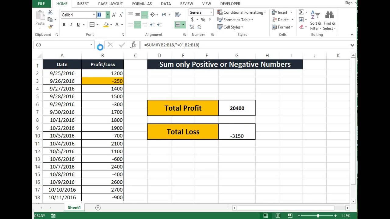
How To Count Sum Only Positive Or Negative Numbers In Excel

I Borrowed An Idea I Found On Here And Through A Google Search I Modified It Slightly To Add On About Positive And 7th Grade Math Math Anchor Charts Line Math

How To Count Sum Only Positive Or Negative Numbers In Excel
How To Format Negative Numbers In Red In Google Sheets Excelnotes
Google Sheets Tips Adding Negative Numbers To Select Cells Youtube
166 Sum Of Negative Values By Months With Two Conditions


How To Show Negative Numbers In Red In Google Sheets

Operations On Positive And Negative Numbers Negative Numbers Anchor Chart Negative Numbers Algebra Help
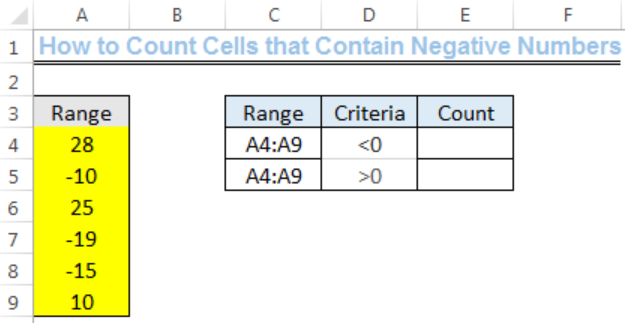
Excel Formula Count Cells That Contain Negative Numbers
How To Format Negative Numbers In Red In Google Sheets Excelnotes
How To Sum Only Positive Numbers Or Only Negative Numbers In Excel 2013 Youtube Youtube

Angles Of Polygons Hidden Picture Polygon Hidden Pictures Angles

How To Show Negative Numbers In Red In Google Sheets
How To Format Negative Numbers In Red In Google Sheets Excelnotes

Pin By Brittany Munoz On Cheat Sheets Integer Rules Algebra Help Math Integers