How To Sum Up A Filtered Column In Excel
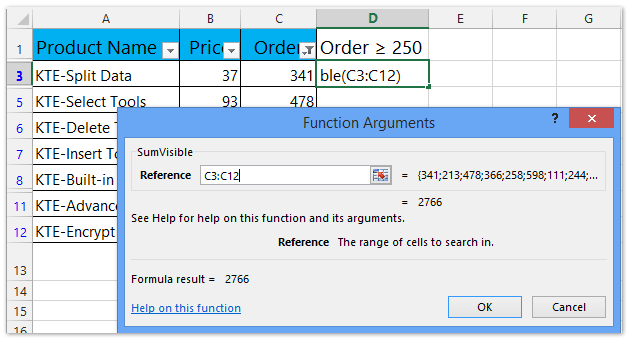
Save this code and enter the formula SumVisible C2C12 into a blank. In the example shown a filter has been applied to the data and the goal is to sum the values in column F that are still visible.

How To Fill Series Of Numbers In A Filtered List Column In Excel
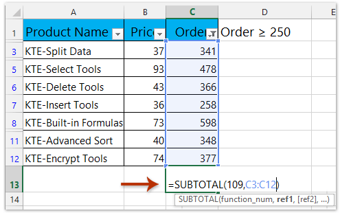
The solution to our problem lies in using the SUBTOTAL Function.
How to sum up a filtered column in excel. The drop-down arrows shown within the red boxes in the. By pressing Alt D F F simultaneously. Hold down the ALT F11 keys and it opens the Microsoft Visual Basic for Applications window.
In case you have data organization so that the cell ranges are separated and you need to SUM all the values in an uninterrupted sequence to the first empty cell then try to use the CSE formulas listed in this tutorial. Finish by clicking the OK button. By filters performing the analysis or any work becomes easy.
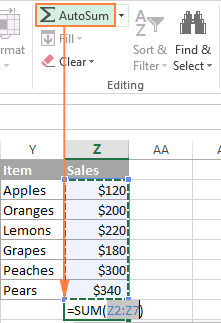
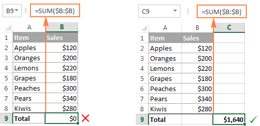
You will see Excel automatically add the SUM function and pick the range with your numbers. Select the data and click filter under the sort and filter drop-down. To avoid any additional actions like range selection click on the first empty cell below the column you need to sum.
There are different ways of applying the Excel column filter. Sum cells based on filter data with certain criteria. Pros of Excel Column Filter.
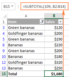
Data menu - Filter. When working with a filtered list in Excel use the SUBTOTAL function instead of SUM to get a total. In the picture below you can see the organization of the data table.
Click the Sort Filter drop down from the Editing group. Excel sum of visible rows. Now from the drop menu of the total sum select the Sum option as shown below.
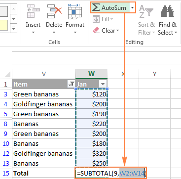
SUMPRODUCTSUBTOTAL3OFFSETB6B19ROWB6B19-MINROWB6B191 B6B19NellyC6C19 B6B19 contains the criteria that you want to use the text Nelly is the criteria and C6C19 is the cell values you want to sum and then press Enter key. The formula used is. A SUBTOTAL formula will be inserted summing only the visible cells in the column.
Click anywhere in the data set. Select the cell where you want the grand total. After that select the cell immediately below the column you want to total and click the AutoSum button on the ribbon.
Just organize your data in table Ctrl T or filter the data the way you want by clicking the Filter button. On Excels Standard toolbar click the AutoSum button or on the keyboard press the Alt key and tap the equal sign key Alt. Click Insert Module and paste the following code in the Module window.
Normally the AutoSum icon inserts a SUM function. 1 2 3 4 5 6 7 8 9 10 11 Function SumVisible. Navigate to the Home tab - Editing group and click on the AutoSum button.
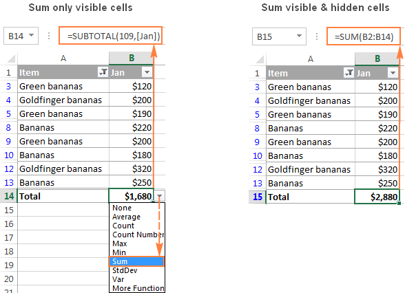
Change the formula from SUM C2C50 to SUBTOTAL 9C2C50 and see the magic. In this example the Region column is filtered for West. With Filter Option Under the Home tab Step 1.
The solution is much easier than you might think. In filtered list SUBTOTAL always ignores values in hidden rows regardless of the function argument. To sum the filtered values in column C based on the criteria please enter this formula.
SUBTOTAL9 F5F14 which returns the sum 954 the total for the 7 rows that are still visible. Click Home from the Ribbon. SUM Filtered Data Using SUBTOTAL Function.
The formula used is. When you apply a filter and then use AutoSum Excel will insert a SUBTOTAL function instead. Because the list is filtered a SUBTOTAL formula is inserted instead of a SUM formula.
Click the drop-down arrow of the. SUBTOTAL9 F5F14 which returns the sum 954 the total for the 7 rows that are still visibleIf you are hiding rows manually ie. The SUBTOTAL function ignores rows hidden by the filte.
In the example shown a filter has been applied to the data and the goal is to sum the values in column F that are still visible. Now go to the top filter drop-down of the same column and select any required colored to get summed up from the Filter by Color option. Specify the ranges to which ignored hidden cells will be summed after opening the Function Arguments dialog box.
The filters are added to the selected data range. How to Sum Up all the values in a sequence up to the first empty cell in the column. Sum visible rows in a filtered list Exceljet.
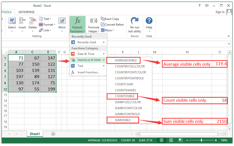
By applying filters we can sort the data as per our needs. By this we enable the table to sum the filtered data as per colored cells. Choose the cell you will place the summing result into and in the Kutools menu choose Functions then Statistical Math SUMVISIBLE or AVERAGEVISBLE COUNTVISIBLE as you wish.
Theres no way for the SUM function to know that you want to exclude the filtered values in the referenced range. By pressing Ctrl Shift L together.

Pivot Table Errors Pivot Table Excel Formula Pivot Table Excel

Ability On Listbox Filtering By Each Column At The Same Time Using A Checkbox Selecting All Items On Listbo Excel Tutorials Excel Spreadsheets Invoice Template
How To Sum Only Filtered Or Visible Cells In Excel
Excel Sum Formula To Total A Column Rows Or Only Visible Cells

How To Count Sum Cells Based On Filter With Criteria In Excel

Using The Subtotal Function To Sum Filtered Data In Excel Microknowledge Inc Excel Excel Shortcuts Data
How To Sum Only Filtered Or Visible Cells In Excel
How To Sum A Column In Excel 5 Easy Ways

Alt Select The Range With The Numbers You Want To Total And Press Enter Column Sum Expense Sheet

A Nice Filtering Template The Value In Textbox Is Searched As Part Or Whole In The Column Visit Link To Download The Samp Excel Computer Help Excel Tutorials
Excel Sum Formula To Total A Column Rows Or Only Visible Cells

How To Stop Pivot Table Columns From Resizing On Change Or Refresh Pivot Table Column Excel
Excel Sum Formula To Total A Column Rows Or Only Visible Cells

Excel Vba Column Copy Excel Tutorials Excel Column

Excel Formula Sum By Group Exceljet

Excel Formula Sum Visible Rows In A Filtered List Exceljet
Excel Sum Formula To Total A Column Rows Or Only Visible Cells
How To Sum Only Filtered Or Visible Cells In Excel
Excel Sum Formula To Total A Column Rows Or Only Visible Cells